Linear regression and implementation in python

The problem statement of any machine learning application can be boiled down to this: we are given some data sets with or without labels attached to them; and we have to formulate a hypothesis function that is closest to the labels of any other samples of data sets that might be given to us at after training our algorithm. 

• Supervised learning: The training data has labels attached to it and can be represented as a tuple $(x_{i},y_{i})$ where i can go from 0 to the number of examples provided (say m) and each $x_{i}$ being an n dimensional vector with each dimension corresponding to features that influence the label y. 
• Unsupervised learning: The training data is unlabeled and represented as ($x_{i}$).

The way we go about building the model in linear regression and most supervised learning algorithms is that some weight $(t_{j})$ is assigned to each dimension of x and a hypothesis function 
$h_{t}(x_{i})$ is calculated. The aim is to solve our machine learning problem like an optimization problem where we evaluate the cost function ( J(t) ) for different values of t and find that particular t value that minimizes the cost function.

$J(t)=\frac{\sum_{m=0}^{m}[h_{t}(x_{i})-y_{i}]^{2}}{2m}$

The hypothesis function (which is fixed for a particular model) for linear regression is given by:

 $h_{t}(x)$=$t_{0}$ + $t_{1}x_{1}$ + $t_{2}x_{2}$ ....+ $t_{n}x_{n}$

It is easier to deal with their vectorized form which reduces the hypothesis function to:

$h_{t}(x)=t'*x$

where $h_{t}$, t and x are n+1 dimensional column vectors and t' is t transpose.

Gradient descent:

One of the optimization techniques that we might use for finding the optimum weight vector is gradient descent. The pseudo code for gradient descent for multivariate linear regression can be written as:

Here $\theta_{j}$ is nothing but the jth weight vector $(t_{j})$ and α is called the learning rate of the algorithm.

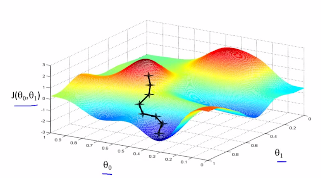
Intuitively, after each iteration the algorithm is traversing in the n dimensional space of the cost function in the direction of descent till it reaches the minima. The magnitude of each step is proportional to the learning rate α and the derivative of the cost function with respect to t. Clearly, gradient descent will converge at the minima when the derivative of the cost function becomes zero.

For effectively applying gradient descent two things should be kept in mind:

• Feature scaling and mean normalization: By feature scaling we mean that all the features should take a similar range of values. Mean normalization means that the mean of all the features should have approximately zero mean. In practice this is done by replacing all xi by (xi-µ)/σ , where µ is the mean and σ is the standard deviation of all the features.

• Choosing the learning rate parameter: If the learning rate parameter is too large the gradient descent might not settle at the global minimum while if it is too small the algorithm will take a lot of time to converge.

Implementation in python using sklearn library:

Here ‘TV’ and ‘Radio’ are two features and Sales is what we are predicting in our data set 'data'. The weight vectors t1, t2 are stored by default in the variable coef_ and t0 is stored in the variable intercept_.

Now that we have trained the weight vectors lets go on to make predictions on the test data set.

R2 score is a statistical parameter that tells us how well a line is fit in our regression model. R2 score of 1 indicates a perfect fit. We are getting an R2 score of 0.897 which is pretty decent. Here we have taken the training set itself as the test set and are finding the rmse between the predicted and the actual value. This does not give us a very accurate idea of our model as it might be over-fitting and not be performing so well on the new test sample that might be given to us.

A better way to build the model is to split training data and reserve some portion of it as test set.

        

Notice that the R2 score has decreased a bit. But a score of 0.86 is still pretty good !